Chapter 14 Dynamic Hamiltonian Monte Carlo and No-U-Turn Sampling (NUTS)
Simulating the Hamiltonian system in HMC provides an extremely efficient means of exploring unimodal target probability distributions. The energy-preservation of the Hamiltonian dynamics means that it is possible to simulate arbitrarily long trajectories in the target space and the corresponding proposals will still be accepted with essentially 100% probability.
In terms of sampling, perhaps the biggest open problem in standard HMC is the choice of the number of steps \(L\) for the Hamiltonian system simulation. The larger the number of steps, the more benefit we will get from HMC through proposing longer moves for the MCMC chain. The caveat is that with too large \(L\), the trajectories will turn back and in many cases will eventually return back to where they started from. With an unfortunate choice of a large \(L\) we may end up in a situation where the algorithm must perform a lot of work to simulate a long trajectory around the target density, only to end up proposing a very short MCMC move.
Another related challenge is that simulating the Hamiltonian system in standard HMC is an all-or-nothing game: if the obtained final state ends up being rejected by Metropolis-Hastings (perhaps the very last step took the simulation to a bad regime), all the work is wasted and the Hamiltonian dynamics simulation needs to start again from scratch.
Dynamic HMC methods address these shortcomings through letting go of the notion of selecting a fixed number of steps \(L\) for the simulation. Instead, the next point in the MCMC chain is chosen dynamically based on the simulated trajectory.
14.1 No-U-Turn Sampling (NUTS)
The No-U-Turn Sampler (NUTS) of Hoffman and Gelman (2014) was the first proposed dynamic HMC algorithm. Intuitively, NUTS works by iteratively extending the simulated trajectory until it observes a U-turn of the path turning back on itself. In order to guarantee reversibility, the path is extended both forward and backward in virtual time. Furthermore instead of a single accept/reject choice, the algorithm samples the next point among the set of candidates generated along the path. The algorithm also includes a heuristic for tuning \(\epsilon\).
14.2 NUTS \(\epsilon\) tuning
In general, too large \(\epsilon\) values lead to unstable leapfrog integration while too small \(\epsilon\) leads to wasted computation.
In NUTS, \(\epsilon\) is tuned by first doubling or halving the value to find an \(\epsilon\) that gives Langevin proposal acceptance rate of approximately 0.5.
This initial guess is further optimised during warm-up iterations toward one achieving the desired target acceptance rate, which can be for example 0.8.
14.3 NUTS sampling
The sampling iteration in NUTS differs from HMC in two respects:
- The simulated trajectory or path in the Hamiltonian system is extended dynamically both forward and backward until a termination condition designed to detect a U-turn is met.
- The next point is sampled from valid alternatives generated during above extension step instead of a single accept/reject choice.
14.3.1 Path extension
The dynamic path extension is illustrated in Fig. 14.1. At step \(j\), the simulation direction (forwards or backwards in time) is chosen randomly and \(2^{j-1}\) leapfrog steps are added to the corresponding end of the path. The evaluated states are stored in a binary search tree as illustrated in Fig. 14.1. This extension of the path both forward and backward is necessary to guarantee the reversibility of the process.
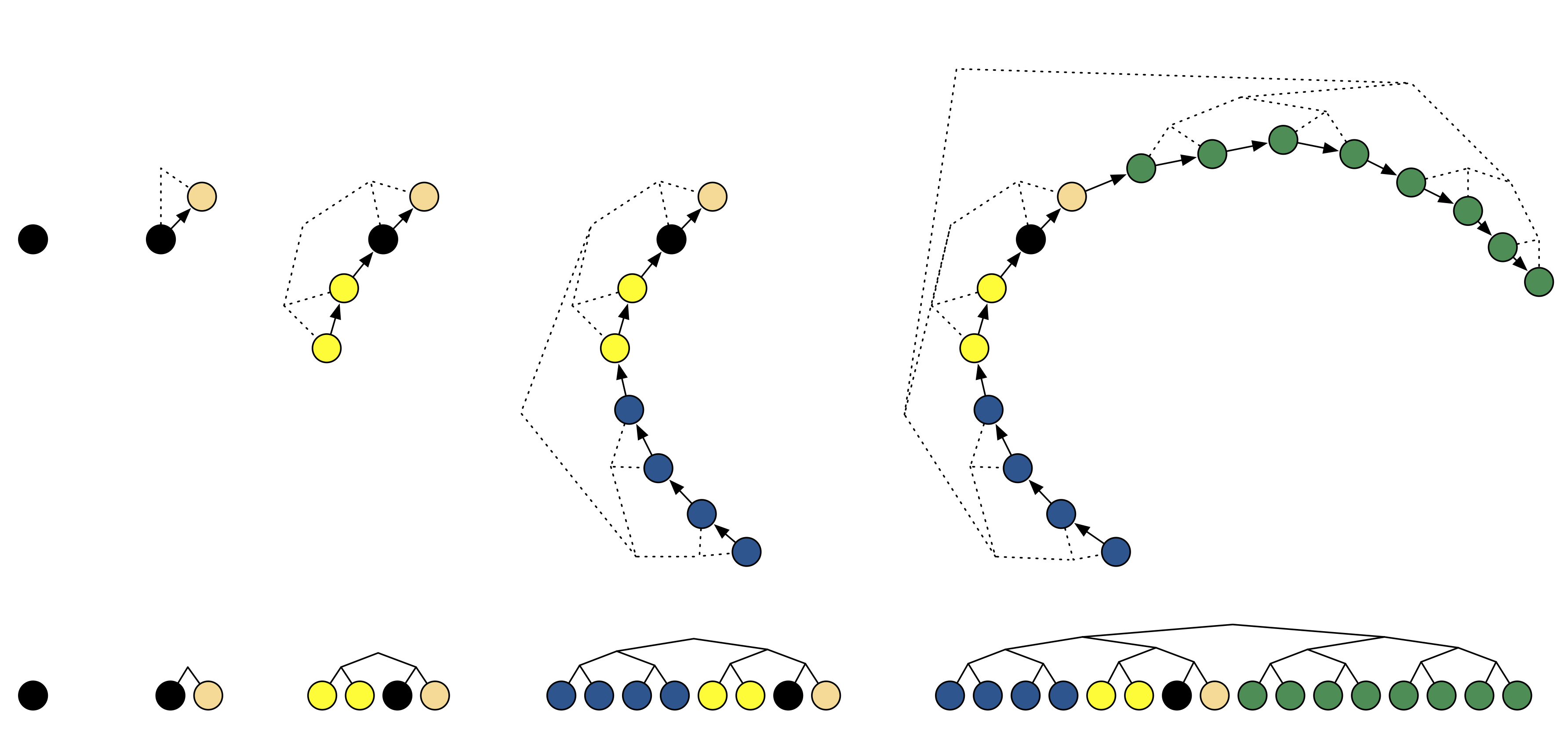
Figure 14.1: NUTS path extension. (Figure from Hoffman and Gelman, 2014.)
The extension process will continue until a termination condition designed to detect a U-turn is met. The condition is based on comparing the current proposal \(\tilde{\mathbf{\theta}}\) and the starting point or initial value \(\mathbf{\theta}\). Looking at the derivative of the squared distance between these points, we can find \[ \frac{\,\mathrm{d}}{\,\mathrm{d} t} \frac{(\tilde{\mathbf{\theta}} - \mathbf{\theta}) \cdot (\tilde{\mathbf{\theta}} - \mathbf{\theta})}{2} = (\tilde{\mathbf{\theta}} - \mathbf{\theta}) \cdot \frac{\,\mathrm{d}}{\,\mathrm{d} t}(\tilde{\mathbf{\theta}} - \mathbf{\theta}) = (\tilde{\mathbf{\theta}} - \mathbf{\theta}) \cdot \tilde{\mathbf{r}}, \] where \(\tilde{\mathbf{r}}\) is the current momentum.
Monitoring when the last quantity becomes negative will tell when the distance starts to decrease, i.e. the simulation has turned back toward the starting point. An example of the termination criterion is illustrated by the arrows at the end of the trajectory in Fig. 14.2.
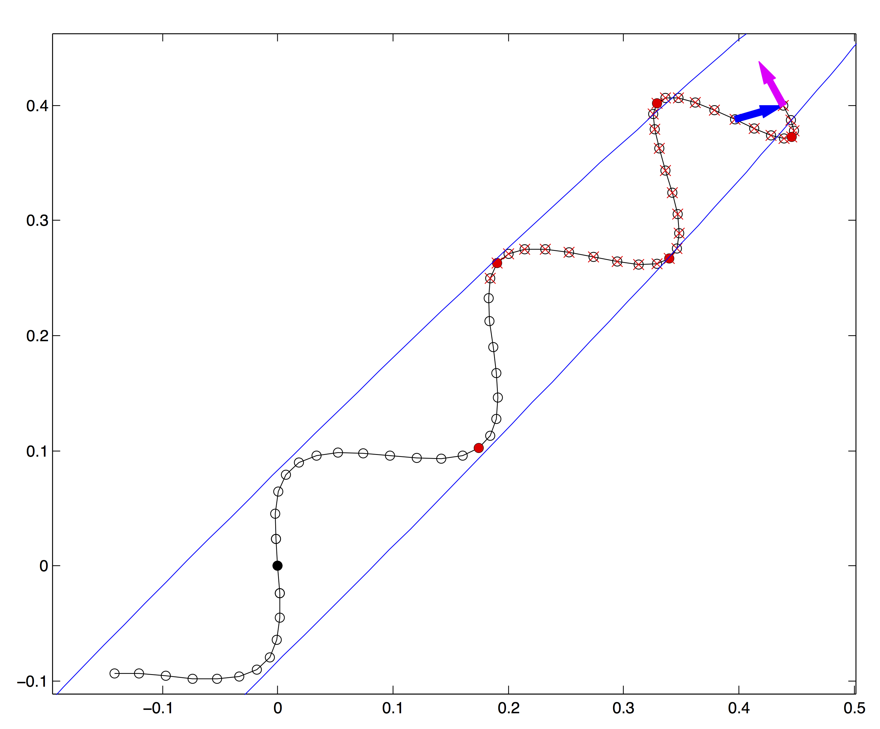
Figure 14.2: NUTS trajectory termination and sample selection. (Figure from Hoffman and Gelman, 2014.)
14.3.2 Sample selection
The other important innovation in NUTS is the selection of the next sample. This procedure needs to be designed carefully to ensure that the resulting sampler satisfies the detailed balance. Because the process does not use Metropolis-Hastings acceptance checks, this needs to be checked and proven separately.
The original NUTS algorithm of Hoffman and Gelman (2014) was based on a method known as slice sampling. In this context, it effectively involves first sampling a rejection energy threshold \[ u \sim \mathrm{Uniform}(0, \exp(- H(\mathbf{\theta}, \mathbf{r}))). \]
To understand the meaning of \(u\), we can take the Metropolis-Hastings acceptance probability for HMC \[ \log a = H(\mathbf{\theta}, \mathbf{r}) - H(\mathbf{\theta}', \mathbf{r}'). \] As usual, the corresponding acceptance check can be realised by simulating \(v \sim \mathrm{Uniform}(0, 1)\) and testing if \[ \log v < H(\mathbf{\theta}, \mathbf{r}) - H(\mathbf{\theta}', \mathbf{r}'). \] By rearranging and exponentiating, this can be formulated equivalently as \[ v \exp(- H(\mathbf{\theta}, \mathbf{r})) < \exp(- H(\mathbf{\theta}', \mathbf{r}')). \] Clearly the LHS of the equation is equivalent to \(u\), meaning the proposal would be accepted if and only if \[ u < \exp(- H(\mathbf{\theta}', \mathbf{r}')).\]
In NUTS, this usual check is further expanded: instead of taking one state and checking if it passes the threshold, a larger number of candidates that pass the threshold are considered and the final sample is chosen by sampling uniformly among the valid candidates. The selection of candidates involves some additional conditions that are presented by Hoffman and Gelman (2014).
14.4 Current development
The quest for the most efficient general purpose MCMC algorithm is not over. Betancourt (2017) notes that the current implementation of NUTS in Stan, which is likely the most efficient at the moment, incorporates a number of refinements over the original algorithm of Hoffman and Gelman (2014), especially in more efficient sample selection via multinomial sampling instead of slice sampling. At the moment these modifications remain unpublished, except for the open source implementation in Stan.
References
Betancourt, Michael. 2017. “A Conceptual Introduction to Hamiltonian Monte Carlo,” January. http://arxiv.org/abs/1701.02434.
Hoffman, Matthew D., and Andrew Gelman. 2014. “The No-U-Turn Sampler: Adaptively Setting Path Lengths in Hamiltonian Monte Carlo.” J. Mach. Learn. Res. 15 (1): 1593–1623. http://www.jmlr.org/papers/volume15/hoffman14a/hoffman14a.pdf.