Chapter 9 Further Monte Carlo techniques and approximate Bayesian computation (ABC)
9.1 Importance sampling
Importance sampling is another general purpose tool for evaluating the expectation of an arbitrary function \(h(x)\) over a difficult density \(f(x)\) by drawing samples from an easy-to-sample surrogate distribution \(g(x)\) and weighting them by the ratio of the true density and the surrogate density.
In equations: \[ I_h = \mathrm{E}_{f(x)}[h(x)] = \int h(x) f(x) \mathrm{d}x = \int h(x) \frac{f(x)}{g(x)} g(x) \mathrm{d}x = \mathrm{E}_{g(x)}\left[h(x) \frac{f(x)}{g(x)}\right]. \]
The corresponding Monte Carlo approximation is \[ I_h \approx \frac{1}{n} \sum_{i=1}^n h(x_i) \frac{f(x_i)}{g(x_i)} = \frac{1}{n} \sum_{i=1}^n h(x_i) w_i, \] where \(x_i \sim g(x)\).
In order to apply importance sampling, it is necessary to have \[ g(x) = 0 \quad \Rightarrow \quad h(x)f(x) = 0. \]
Good importance sampling estimators have low variance. In particular, it is important that the variance is finite, which requires that \[ \mathrm{E}_g\left[ h^2(x) \frac{f^2(x)}{g^2(x)} \right] = \int h^2(x) \frac{f^2(x)}{g(x)} \mathrm{d}x < \infty. \] This is guaranteed for example if \[ \mathrm{Var}_f[h(X)] < \infty, \quad \text{and} \quad \frac{f(x)}{g(x)} \le M, \forall x\] for some \(M > 0\).
9.2 Likelihood-free inference and approximate Bayesian computation (ABC)
MCMC and other common inference methods provide methods for models where we can compute the likelihood \(p(\mathcal{D} | \theta)\). This class of models is large, but it does not include all models that are of practical interest. Phylogenetic tree models and certain dynamical models with stochastic differential equations involve likelihoods that are computationally intractable: they may for example require computing a normalisation factor over a very large space.
Instead of depending on the likelihood, so called likelihood-free inference methods are based on simulating new synthetic data sets. For many models, this simulation may be easier than evaluating or even defining a likelihood. The inference is then based on comparing the simulated synthetic data sets with the observed data set.
9.3 Approximate Bayesian computation (ABC)
Let us consider a model \(p(\mathcal{D}, \theta) = p(\mathcal{D} | \theta) p(\theta)\) for some data \(\mathcal{D}\) that depends on some parameter \(\theta\).
The basic idea of ABC is very simple:
- Sample \(\theta^* \sim p(\theta)\) from the prior \(p(\theta)\)
- Simulate a new observed data set \(\mathcal{D}^*\) conditional to \(\theta^*\): \(\mathcal{D}^* = \eta(\theta^*) \sim p(\mathcal{D} | \theta^*)\).
- Accept or reject the sample according to criteria specified below.
9.4 Exact rejection ABC
In exact rejection ABC, a simulated sample \(\theta^*\) is accepted if and only if \(\mathcal{D}^* = \mathcal{D}\). In this case it is easy to see that the accepted samples follow the posterior distribution \(p(\theta | \mathcal{D})\).
Exact rejection ABC is only applicable to very simple problems, because usually the probability of simulating an exact replica of the data set is negligible.
9.5 Summary statistics ABC
ABC can be made more efficient by requiring that only some summary statistics \(S(\mathcal{D})\) should match between the generated and the observed data sets. These could be e.g. means and variances of the data. In case the selected statistics are sufficient, such as mean and variance for the normal distribution, the sampler will still be exact.
Summary statistics allow for a simple relaxation that makes the sampler approximate: we can accept proposals with \[ \| S(\mathcal{D}) - S(\mathcal{D}^*) \| < \epsilon \] for some \(\epsilon > 0\). This can make sampling significantly more efficient, especially in the case of continuous \(\mathcal{D}\) and \(S(\mathcal{D})\), at the cost of sampling from an approximation of the posterior.
9.6 What is approximate ABC sampling from?
Dropping sufficient statistics for a moment, the above approximate procedure of accepting samples with \(\| \mathcal{D} - \mathcal{D}^* \| < \epsilon\) can be generalised to a procedure where the proposed sample \(\theta^*\) is accepted with probability \[ a = \frac{\pi_{\epsilon}(\mathcal{D} - \mathcal{D}^*)}{c}, \] where \(\pi_{\epsilon}(\cdot)\) is a suitable probability density and the constant \(c\) is chosen to guarantee that \(\pi_{\epsilon}(\mathcal{D} - \mathcal{D}^*)/c\) defines a probability.
Applying ABC with this acceptance probability can be shown (Wilkinson (2013)) to be equivalent to sampling from the posterior distribution of the model \[ \mathcal{D} = \eta(\theta) + \epsilon, \] where \(\epsilon \sim \pi_{\epsilon}(\cdot)\) is independent of \(\eta(\theta)\).
Thus ABC sampling with a non-zero \(\epsilon\) is equivalent to sampling from the posterior of a related model that incorporates and extra noise term.
9.7 ABC example
Let us simulate 1000 draws from the posterior of the binomial model \[ p(x | n, \pi) = \mathrm{Binomial}(x;\;n, \pi) \] used to simulate the number of heads on \(n\) coin flips where the unknown probability of heads is \(\pi\) with prior \[ p(\pi) = \mathrm{Uniform}(0, 1). \]
import numpy as np
import numpy.random as npr

def abc_coinflip(N, n, k):
    samples = np.zeros(N)
    nsamples = 0
    while nsamples < N:
        p = npr.uniform()
        if npr.binomial(n, p) == k:
            samples[nsamples] = p
            nsamples += 1
    return samples

samples = abc_coinflip(1000, 20, 10)
h = plt.hist(samples, 30, density=True)
plt.show()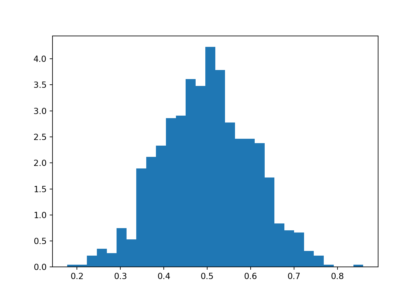
9.8 Further developments
Even after allowing for some slack in the match of the summary statistics, independent sampling from the prior may be too inefficient. Methods coupling ABC with some form of MCMC or otherwise learning where to sample the proposals can help.
ABC is often presented in scientific contexts in combination with simulators of physical or chemical systems, such as simulators of epidemics caused by contagious pathogens. The ABC approach allows combining the knowledge built into these simulators with Bayesian inference.
ABC bears clear conceptual similarity with generative adversarial networks (GANs) that are widely used in machine learning with deep neural networks. GANs employ a combination of two neural networks: a generator and a discriminator. GAN learning is based on a game where the generator attempts to generate synthetic samples that would be indistinguishable from real data while the discriminator tries to distinguish these. The sampling performed in ABC based on similarity of the generated and true data can be seen as a kind of probabilistic variant of GANs.
References
Koistinen, Petri. 2013. “Computational Statistics.”
Sunnåker, Mikael, Alberto Giovanni Busetto, Elina Numminen, Jukka Corander, Matthieu Foll, and Christophe Dessimoz. 2013. “Approximate Bayesian Computation.” PLoS Computational Biology 9 (1): e1002803. https://doi.org/10.1371/journal.pcbi.1002803.
Wilkinson, Richard. 2013. “Approximate Bayesian Computation (ABC) Gives Exact Results Under the Assumption of Model Error.” Stat. Appl. Genet. Mol. Biol. 12 (2). https://arxiv.org/abs/0811.3355.
Wilkinson, Richard, and Simon Tavaré. 2008. “Approximate Bayesian Computation: A Simulation Based Approach to Inference.” http://www0.cs.ucl.ac.uk/staff/C.Archambeau/AIS/Talks/rwilkinson_ais08.pdf.