Chapter 4
Machine learning as minimization of errors
In this chapter, we will go through some of the basics of the backbone of modern AI: machine learning. Such AI
crucially relies on learning from incoming data, which is also true of the brain. Machine learning is
most often used in conjunction with neural networks, which are powerful function approximators,
loosely mimicking how computations happen in the brain. We will also consider an alternative,
older approach to intelligence based on symbols, logic, and language, which is now called “good
old-fashioned AI”. (The preceding chapter with its discrete, finite states, was an example of this latter
approach.)
A central message in this chapter is that learning is often based on some measure of error. Minimizing such
errors means optimizing the performance of the system. The fundamental importance of computing and
signalling such errors is important in future chapters where such errors are directly linked to suffering,
generalizing the concept of frustration. I conclude this chapter by claiming that any kind of learning
from complex data can lead to quite unexpected results, something that the programmer could not
anticipate.
Neurons and neural networks
Modern AI is based on the observation that the human brain is the only “device” we know to be intelligent for sure and
without any controversy. It is actually not easy to define what “intelligence” means, and I will not attempt to do that
in this book.
Yet, nobody denies that the brain is intelligent—or, to put it another way, it enables us to behave in an
intelligent way. The brain is intelligent as if by definition; it is the very standard-bearer of intelligence. If you
want to build an intelligent machine, it makes sense to try to mimick the processing taking place in the
brain.
Neurons as tiny processors
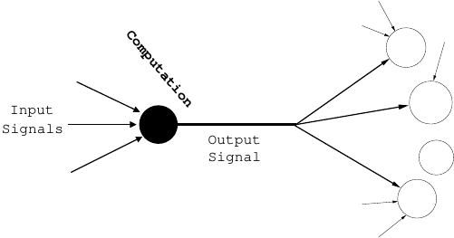
The computation in the brain is done by specialized cells called neural cells or neurons. A schematic picture of a
neuron is in Fig. 4.1. A neuron receives input from other neurons, processes that input, and outputs
the results of its computations to many other neurons. There are tens of billions of neurons in
the human brain. Each single neuron can be seen as a simple information-processing unit, or a
processor.
All these tiny processors do their computations simultaneously, which is called parallel processing in
technical jargon. The opposite of parallel processing is serial processing, where a single processor does various
computational operations one after another—this is how ordinary CPU’s in computers work. Another major
difference between the brain and ordinary computers is that processing in neurons is also distributed. This means
that each neuron processes information quite separately from the others: It gets its own input and
sends its own output to other neurons, without sharing any memory or similar resources. Compared
to an ordinary PC, the brain is thus a massively parallel and distributed computer. Instead of a
couple of highly sophisticated and powerful processors as found in a PC, the brain has a massive
amount—billions—of very simple processors. (Parallel and distributed processing is discussed in detail in
Chapter 6.)
While the actual neurons are surprisingly complex, in AI, a highly simplified model of a real neuron is
used. Sometimes, such a model is called an artificial neuron to distinguish it from the real thing,
but for simplicity, we call them just neurons. Like a real neuron, an artificial neuron gets input
signals from other neurons, but each such input signal is very simple, just a single number; we can
think of it as being between zero and one, like a percentage. Based on those inputs, the neuron
computes its output which is, again, a single number. This output is, in its turn, input to many other
neurons.
In such a simple model, the essential thing is to devise a simple mathematical formula for computing the
output of the cell as a function of the inputs. In typical models, the output is computed, essentially, as a
weighted sum of the inputs. The weights used in that sum are interpreted, in the biological analogy, as the
strengths of the connections between neurons, or the incoming “wires” on the left-hand-side of Fig. 4.1. These
weights can get either positive or negative values: The weight is defined as zero for those neurons from which no
input is received. The weighted sum is usually further thresholded (i.e. passed through a nonlinear function) so
that the output is forced to be between zero and one. In the brain, the connections are implemented
through small communication channels called synapses, which is why the weights can also be called
“synaptic”.
Importantly, these weights can be interpreted as a pattern, or a template, which the neuron is sensitive to.
Thus, a neuron can be seen as a very simple pattern-matching unit. The neuron gives a large output if the
pattern of all the input signals matches the pattern stored in the vector of weights or connection
strengths.
As an illustration, consider a neuron which has a weight with the numerical value +1 for inputs from
another neuron, let’s call it neuron A, as well as a zero weight from neuron B, and a weight of -1
neuron C. This neuron will give a maximal output (it is maximally “activated”) when the input to
the neuron is similar to the pattern of those weights: It will output strongly when neuron A gives
a large output and the neuron C has a small output, while it does not care what the output of
neuron B might be. In other words, the neuron computes how well the pattern stored in its synaptic
weights matches with the pattern of incoming input, and its output is simply a measure of that
match.
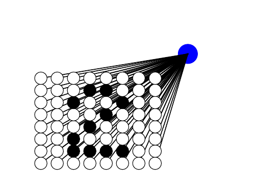
Such pattern-matching is obviously most useful in processing sensory input, such as images. Consider a
neuron whose inputs come from single pixels in an image. That is, the input consists of the numerical
values of each pixel, telling how bright it is, i.e. whether it is white, black, or some sort of grey.
Then, we can plot the synaptic weights as an image, so that the grey-scale value in each pixel in
this plot is given by the corresponding synaptic weights. If they are -1 or +1 as in the previous
example, we can plot those values as black and white, respectively. A neuron could have synaptic
weights as in Fig 4.2. Clearly, this neuron is specialized for detecting a digit, in particular number
two.
Of course, in reality, to recognize digits (or anything else) in real images, things are much more complicated.
For one thing, the pattern to be recognized could be in a different location. If the digit is moved just one pixel to
the right or to the left, the pattern matching does not work anymore, and the neuron will not recognize the
digit. Likewise, if the digit were white on a black background instead of black on a white background,
the same pattern-matching would not work. To solve these problems, we need something more
sophisticated.
Networks based on successive pattern matching
Building a neural network greatly enhances the capabilities of such an AI, and solves the problems just
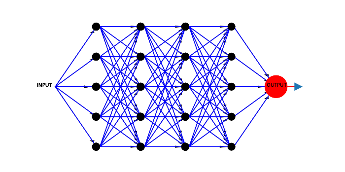
mentioned. A neural network is literally a network consisting of many neurons. Networks can take many different
forms, but the most typical one is a hierarchical one, where neurons are organized into layers, each of which
contains several cells, actually quite a few sometimes. The incoming input first goes to the cells in the first layer
which compute their outputs and send them to neurons in the second layer, and so on. This is illustrated in
Figure 4.3.
From the viewpoint of pattern-matching, such a network performs successive and parallel pattern matching.
The input is first matched to all the patterns stored in the first-layer neurons, and those neurons then output the
degrees to which the input matched their stored patterns or templates. These outputs are sent to the next layer,
whose neurons then compare the pattern of first-layer activities to their templates. So, the second-layer patterns
are not patterns of original input (such as the pixels of an image) but patterns of the first-layer activities,
which form a description of the input on a slightly more abstract level. This goes on layer by layer,
so that each neuron in each layer is “looking for” a particular kind of pattern in the activities of
the neurons in the previous layer. The patterns are always stored in the synaptic weights of the
neurons.
The utility of such a network structure is that it enables much more powerful computation. For example,
consider the problem of a digit which could be in slightly different locations in the image, as mentioned above.
The problem of different locations can be fixed by having several neurons in the first layer, each of
which matches the digit in one possible location. All we need in the second layer is a neuron that
adds the inputs of all first-layer neurons, and thus computes if any of them finds a match. With
such a scheme, the second-layer neuron is able to see if there is a digit “2” at any location in the
image.
Finding the right function by learning
Now, a crucial question is how the synaptic connection weights can be set to useful values. In modern AI, the
synaptic weights between neurons are learned from data, hence the term machine learning. Learning is really the
core principle in most modern AI. Especially in the case of neural networks, it is actually difficult to imagine any
alternative. How could a human programmer possibly understand what kind of strengths are needed between the
different neurons? In some cases, it might be possible: in image processing, the first one or two layers do have
rather simple intuitive interpretations, as we have alluded to above. However, with many layers—and neural
networks can have thousands of them— the task seems quite impossible, and hardly anybody has seriously tried
to design such neural networks by fixing the weights manually, based either on some theory or
intuition.
In the brain, the situation is quite similar. There is simply not enough information in the genome—which is
somewhat analogous to the programmer here—to specify what the synaptic connection strengths should be for
all the neurons. It would hardly be optimal anyway to let the genes completely determine the synaptic
connections, since animals live in environments that may change from one generation to another, and
some individual adaptation to circumstances is clearly useful. What happens instead is that the
synaptic weights change as a function of the input and the output of the neuron, or as a function of
perceptions and actions of the organism. The capability of the brain to undergo such changes is called
“plasticity”, and those changes are the biophysical mechanism underlying most of learning in humans or
animals.
How such changes precisely happen in the brain is an immensely complex issue, and we understand only
some basic mechanisms. Nevertheless, in AI, a number of relatively simple and very useful learning algorithms
have been developed. Neural networks using them learn to perform basic “intelligent” tasks such as recognizing
patterns (is it a cat or a dog?) or predicting the future (if I turn left at the next intersection, what will I see?).
Learning in a neural network in such a case is based on learning a mapping, or function, from input data to
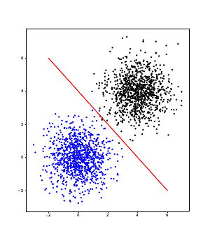
output data. Let’s first consider a single neuron. It can basically learn to solve simple classification problems, as
illustrated in Figure 4.4. If the classes are nicely separated in the input space, a single neuron
can learn, as its synaptic weights, the pattern that precisely describes the difference between the
classes.
However, a network with many neurons can learn to represent much more complex functions from input to
output. The input data could be photographs and the output data could be a word describing the main content
of the photograph (“cat”, “dog”, or “unicorn”). The learning of the input-output mapping then consists of
changing the synaptic weights of all the neurons in all the layers. In successive layers, the network performs
increasingly sophisticated and abstract computations, consisting of matching the inputs successively to the
templates given by the weight vectors in each layer. After learning the right mapping, you can input a
photograph to the system, and the output of the neural network will give its estimate of what the photograph
depicts.
There is an infinite number of different ways you can use a neural network by just defining the inputs and
outputs in different ways. If you want to learn to predict future stock prices, the input data would be
the past prices and the output, current stock prices. You can create a recommendation system
that recommends new products to people in online shopping by defining the inputs to be some
personal information of the customers, and the output whether the customer bought a certain item or
not.
In a rather unsavoury application, the inputs would be what a social media user likes, and the
output some sensitive personal information (say, sexual orientation), and then you can predict
that sensitive information for anybody. Whether the prediction is accurate is another question, of
course.
Here, we see one main limitation of machine learning: The availability of data. Where do you get the
sensitive personal information of social media users in the first place, i.e. where do you get the data to train
your network? Maybe nobody wants to give you such sensitive data. In other cases, the data may be very
expensive to collect; for example, in a medical application, useful measurements and their analyses may cost a
lot of money. Finding suitable data is a major limiting factor in neural network training; this is a theme we will
come back to many times. Learning needs data, obviously; but it also needs the right kind of data, and enough
of it.
Learning as minimization of errors
After we have got the data, we need to define how to actually perform the learning. Most often, the learning is
based on formulating some kind of error, and the network then tries to minimize it by an algorithm. The error is
a function of the data, i.e. something that can be computed based on the data at our disposal, and tells us
something about how well the system is performing.
Suppose the data we have consists of a large number of photographs and the associated categories (cat/dog
etc.). To recognize patterns in the images, the network could learn by minimizing the percentage of input
images classified incorrectly, called classification error. Alternatively, suppose we want to learn
to predict how an agent’s actions change the world—say, how activation of an artificial muscle
changes the position of the arm of a robot. In that case, what is minimized is prediction error: The
magnitude of the difference between the predicted result of the action and the true result of the
action (which can be observed after the action). Such errors don’t usually go to zero, i.e. there will
always be some error left even after a lot of learning. This is due to the uncertain and uncontrollable
nature of the world and an agent’s actions; that’s another theme we will discuss in detail in later
chapters.
We also need to develop an algorithm to minimize the errors, but there are standard solutions that usually
are satisfactory. What most such algorithms have in common is they learn by making tiny changes in the weights
of the networks. This is because optimizing an error function, such as classification error, is actually a very
difficult computational task: There is usually no formula available to compute the best values for the weight
vectors. In contrast, what is usually possible is to obtain a mathematical formula that gives the
direction in which the weights should be changed to make the error function decrease the fastest. That
direction is given by what is called the gradient, which is a generalization of the derivative in basic
calculus.
So, you can optimize the error function step by step as follows. You start by assigning some random values to
the weight vectors. Given those values, you can compute the gradient, and then take a small step in that
direction (i.e. move the weight vector a bit in that direction), which should reduce the error function, such as
prediction error. But you have to repeat that many times, often thousands or even millions, always computing
the gradient for the new weight values obtained at the previous step. (The direction of the gradient is different
at every step unless the error function is extremely simple.) Such an algorithm is called iterative (repeating)
because it is based on repeating the same kind of operations many times, always feeding in the results of the
previous computation step to the next step. Using an iterative algorithm may not sound like a very efficient way
of learning, but usually an iterative gradient algorithm is the only thing we are able to design and
program.
Such an algorithm is a bit like somebody giving you instructions when you’re parking your car and cannot
see the right spot precisely enough. They will only give instructions which are valid for a small displacement.
When they say “Back”, that means you need to back the car a little bit, and then follow some new instructions.
This is essentially an iterative algorithm, where you get instructions for the direction of a small displacement,
and they are different at every time step.
Neural networks use an even more strongly iterative method, based on computing the gradient for just a few
data points at a time. A data point is one instance of the input-output relation data, for example, a single
photograph and its category. In principle, a proper gradient method would look at all the data at its disposal,
and push the weights a small step in the direction that improves the error function, say the classification error,
for the data set as a whole. However, if we have a really big data set, say millions of images, it may be too
slow to compute the error function for all of them. What the algorithms usually do is to take a
small number of data points and compute the gradient only for those. That is, you just take a
hundred photographs, say, and compute the gradient, i.e. in which direction the weights should
be moved to make the classification accuracy better, for those particular images. Importantly, at
every step you randomly select a new set of a hundred images, and do the same thing for those
images.
The point is that you are still on average moving the weights in the right direction, so this is not much worse
than computing the real gradient. But crucially, you can take steps much more quickly, since the computation
of the gradient is much faster for the small sample. It turns out that in practice, the benefit of
taking more steps often overwhelms the slight disadvantage of having just an approximation of the
gradient.
Putting these two ideas together, we get what is called the stochastic gradient descent algorithm. Here,
“descent” refers to the fact that we want to minimize an error. “Stochastic” means “random”, and refers to the
fact that you are computing the gradient for randomly chosen data points, so you are going in the right direction
only on average.
Suppose you’re in an unfamiliar city and you need to get to the railway station. Your “error function” is the
distance from the station. You can ask a passer-by which direction the station is, and you get something
analogous to the gradient for one data point. Now, of course, that direction given by the passer-by is not certain,
she could very well be mistaken; maybe she even said she is not quite sure about the direction. But you
probably prefer to walk a bit in that direction, and then ask another passer-by. This is like stochastic
gradient descent, where you follow an approximation of the gradient, given by each single data
point. The opposite would be that instead of following each person’s advice one after the other,
you first ask everybody you see on the street where they think the station is, and move in the
average of the directions they are giving. Sure, you would get a very precise idea of what the right
direction is, but you would advance very slowly—this is analogous to using the full, non-stochastic
gradient.
Gradient optimization vs. evolution
There are many more ways of optimizing an error function, and many systems that can be conceptualized as the
optimization of a function. In particular, evolution is a process where the error function called fitness is optimized.
Fitness is basically the same as reproductive success, which can be quantified as the expected number of offspring of an
organism.
Fitness is, of course, maximized, while errors in AI are minimized. However, this difference is completely
insignificant on the level of the optimization algorithms, since maximization of a function is the same as
minimizing the negative of that function. Thus, evolution can equally well be seen as minimization of the
negative fitness.
In general, such a function to the optimized—whether minimized or maximized—is called an “objective
function”. The objective function does not necessarily have to be any kind of a measure of an error, although in
AI, it often is. Note that the objective function is different from the function from the input to the output
that the neural network is computing, as described above. The objective function is what enables
the system to learn the best possible input-output function, so it works on a completely different
level.
Evolution works in a very different way than stochastic gradient descent. But it is actually possible to
mimick evolution in AI and use what is called evolution strategies, evolutionary algorithms, or genetic
algorithms. These are iterative algorithms which are sometimes quite competitive with gradient methods. They
can optimize any function, which does not need to have anything to do with biological fitness. For example, we
can learn the weights in a neural network by such methods. The idea is to optimize the given error function by
having a “population” of points in the weight space, which is like a population of individual organisms in
evolution.
Like real evolution, such algorithms are based on two steps. First, new “offspring” is generated for each
existing “organism”. In the simplest case, you randomly choose some new weight values close to the current
weight values of each organism, which is a bit like asexual reproduction in bacteria, with some mutations to
create variability. Then, you evaluate each of those new organisms by computing the value of the error (such as
classification error) for their values for weights. Finally, you consider the value of the error as an analogue of
fitness in biological evolution, albeit with the opposite sign because fitness is to be maximized while an error
function is to be minimized. What this means is that you let those organisms (or weight values) with the
smallest values of the error “survive”, i.e. you keep those weight values in memory and discard those weight
values which have larger (that is, worse) values of the error function. You also discard the organisms
of the previous iteration or “generation”, since those individual organisms die in the biological
analogy.
Such an evolutionary algorithm will find new weight values which are increasingly better because only the
organisms with the best weight values survive in each iteration. Thus, it is an iterative algorithm that optimizes
the error function. It is a randomized algorithm, like stochastic gradient descent, in the sense that it randomly
probes new points in the weight space. In fact, an evolutionary algorithm is much more random than stochastic
gradient descent, since gradient methods use information about the shape of the error function to find the best
direction to move to, while evolutionary methods have no such information. This is a disadvantage of
evolutionary algorithms, but on the other hand, one step in an evolutionary algorithm can be much
faster to compute since you don’t need to compute the gradient, just random variations of existing
weights.
So, we see that both evolution and machine learning are optimizing objective functions. The optimization
algorithms are often quite different, but they need not be. One important difference is that in machine learning,
the programmer knows the error function, and explicitly tells the agent to minimize it. In real biological
evolution, fitness is an extremely complicated function of the environment; it cannot be computed by anybody,
nor can its gradient. Real biological fitness can only be observed afterwards, by looking at who survived in the
real environment, and even then you only get a rough idea of the values of fitness of the individual organisms
concerned: Those who die probably had a low fitness, but it is all quite random—even more than stochastic
gradient descent. (If an organism were actually able to compute the gradient of its fitness, that would
give it a huge evolutionary advantage.) Another important difference is that in biology, evolution
works on a very long time scale, over generations, while in AI, the learning in the neural networks
happens typically inside an individual’s life span. The evolutionary algorithms in AI typically learn
within an individual agent’s lifespan as well, only simulating “offspring” of a neural network in its
processors.
Learning associations by Hebbian rule
So far, we have seen learning as based on finding a good mapping from input to output. Such learning is called
supervised because there is, metaphorically speaking, a “supervisor” that tells the network what the right output
is for each input. Yet, sometimes it is not known what the output of a neural network should be, or whether
there is any point at all in talking about separate input and output—especially if we are talking about the brain.
In such a case, learning needs to be based on completely different principles, called unsupervised learning.
In unsupervised learning, the learning system does not know anything about any desired output
(such as the category of an input photo). Instead, it will try to learn some regularities in the input
data.
The most basic form of unsupervised learning is learning associations between different input items. In a
neural network, they are represented as connections between the neurons representing those two items. For
example, if you have one neuron representing “dog” and another neuron representing “barking”, it is reasonable
that there should be a strong association between them.
One theory of how such basic unsupervised learning happens in the brain is called Hebbian learning. Donald
Hebb proposed in 1949 that when neuron A repeatedly and persistently takes part in activating neuron B,
some growth process takes place in one or both neurons such that A’s efficiency in activating B is
increased.
Such Hebbian learning is fundamentally about learning associations between objects or events. A
very simple expression of the Hebbian idea is that “cells that fire together, wire together”,
where “firing” is a neurobiological expression for activation of a neuron. In this formulation,
Hebbian learning is essentially analysing statistical correlations between the activities of different
neurons.
One thing which clearly has to be added to the original Hebbian mechanism is some kind of
forgetting mechanism. It would be rather implausible that learning would only increase the
connections between neurons. Surely, to compensate, there must be a mechanism for decreasing the
strengths of some connections as well. Usually, it is assumed that if two cells are not activated
together for some time, their connection is weakened, as a kind of negative version of Hebb’s
idea.
Hebbian learning has been widely used in AI, and it has turned out to be a highly versatile tool. You can
build many different kinds of Hebbian learning, depending on how the inputs are presented to the system and on
the mathematical details of how much the synaptic strengths are changed as a function of the firing rates. You
can also derive Hebbian learning as a stochastic gradient descent for some specially crafted error
functions.
Logic and symbols as an alternative approach
The inspiration for neural networks is that they imitate the computations in the brain. Since the brain is
capable of amazing things, that sounds like a good idea. But historically, before neural networks, the
initial approach to AI was quite different. It was actually more like the world of planning we saw in
Chapter 3, where the world states are discrete, and there are few if any continuous-valued numerical
quantities.
In early AI, it was thought that logic is the very highest form of intelligence, and therefore, AI should be
based on logic. Also, the principles of logic are well-known and clearly defined, based on hundreds of years of
mathematics and philosophy, so they should provide, it was thought, a solid basis on which to build
AI. In modern AI, such logic-based AI is not very widely used, but it is making a come-back: It
is increasingly appreciated that intelligence is, at its best, a combination of neural networks and
logic-based AI—now called “good old-fashioned” AI, or GOFAI for short. Such logic provides a form of
intelligence that is in many ways completely different from neural network computations, as we will see
next.
Binary logic vs continuous values
Mathematical logic is based on manipulating statements which are connected by operators such
as AND and OR. For example, a robot might be given information in the form of a statement
that “the juice has orange colour AND the juice is in the fridge”. Any statement can also be made
negative by the NOT operator. An important assumption is such systems, in their classical form,
is that any statement is either true or false; no other alternatives are allowed. This goes back to
Aristotle and is often called the law of the “excluded third”. That is, truth values are binary (have two
values).
Such logic is perfectly in line with the basic architecture of a typical computer. Current computers operate
on just zeros and ones, and those zeros and ones can be interpreted as truth values: Zero is false and one is true.
Such computers are also called “digital”, meaning that they process only a limited number of values, in this case
just two. Our basic planning system in the preceding chapter, with its finite number of states of the world, was
an example of building AI with such a discrete approach, and planning is fundamentally based on logical
operations.
The brain, in contrast, computes with quantities which are in “analog” form, which means the
continuous-valued numbers, which take a potentially infinite number of possible values. Artificial neural
networks do exactly the same, as they are trying to mimick even this aspect of the brain. It is
rather unnatural for the brain to manipulate binary data or to perform logical operations. It is
possible only due to some very complex processes which we do not completely understand at the
moment.
This distinction between digital and analog information-processing is another important difference between
ordinary computers on the one hand, and the real brain or its imitation by neural networks on the other.
(Earlier we saw the distinction between parallel and distributed processing in the brain versus the serial
processing in an ordinary computer.) The digital nature of ordinary computers implies that any data that you
input has to be converted to zeros and ones. This is actually a bit of a problem because a lot of data in the real
world does not really consist of zeros and ones. For example, images are really intensities of light at different
wavelengths, measured in a physical unit called “lux”. One pixel in an image might have an intensity of 1,536
lux and another 5,846 lux. It is, again, rather unnatural to represent such numbers using bits, which is why
processing non-binary data such as images is relatively slow in modern computers, compared to binary
operations.
Categories and symbols
Saying that things are either true or false is related to thinking in terms of categories. Human thinking is largely
based on using categories: We divide all the perceptual input—things that we see, hear, etc.—into classes with
little overlap. Say, you divide all the animals in your world into categories such as cats, dogs, tigers, elephants,
and so on, so that each animal belongs to one category—and usually just one. Then, you can start talking about
the animals in terms of true and false. You can make a statement such as “Scooby is a dog”, and that is either
true or false based on whether you included that particular animal in the dog category; any other (third) option
is excluded.
Categories are usually referred to by symbols, which in AI are the equivalent of words in a human language.
For example, we have a category referred to by the word “cat”, which includes certain “animals” (that’s another
category, actually, but on a different level). Ideally, we have a single word that precisely corresponds to each
single category, like the words “cat” and “animal” above. Such symbols are obviously quite arbitrary since in
different languages the words are quite different for the same category. An AI system might actually just use a
number to denote each category.
We see that logic-based processing goes hand-in-hand with using categories, which in its turn leads to what is
sometimes called symbolic AI. These are all different aspects of GOFAI.
From hand-coded logic to learning
Historically, one promise of GOFAI was to help in medical diagnosis, where the programs were often called
“expert systems”. This sounds like a case where categories must be useful since medical science uses various
categories referring to symptoms (“cough”, “lower back pain”) as well as diagnoses (“flu”, “slipped
disk”).
The basic approach was that a programmer asks a medical expert how a medical diagnosis is made, and then
simply writes a program that performs the same diagnosis, or makes the same “decisions” in the technical
jargon. For example, one decision-making process by the human expert might be translated into a formula such
as
IF cough AND nasal congestion AND NOT high fever THEN diagnosis is common cold
However, this research line soon ran into major trouble. The main problem was that medical doctors, and
indeed most human experts in any domain, are not able to verbally express the rules they use for
decision-making with enough precision. This is rather surprising since we are operating with human
language and well-known categories. The situation is different from neural networks where it is
intuitively clear that no expert can directly tell what the synaptic weights should be, because their
workings are so complex and counterintuitive. Yet, it turned out that even medical diagnoses are often
based on intuitive recognition of patterns in the data, which is a form of tacit knowledge. Tacit
knowledge means knowledge, or skills, which cannot be verbally expressed and communicated to
others.
A major advance in such early AI was to understand that expert systems should actually learn the decision
rules based on data. Again, learning provides a route to intelligence that is more feasible than trying to directly
program an intelligent system. Given a database with symptoms of patients together with their diagnoses given
by human experts, a machine learning system can learn to make diagnoses. Such learning is not so
fundamentally different from learning by neural networks. What is different is that the data is categorical
(“cough”, “no cough”), and the functions are computed in a different way, for example by combining logical
operations such as AND, OR, and NOT.
Categorization and neural networks
By definition, such logic-based AI can only learn to deal with data which is given as well-defined categories. Yet,
real data is often given as numbers instead of categories; even medical input variables often include numerical
data in the form of lab test results. In this medical diagnosis, we have indeed a category called “high fever”. The
system is effectively dividing the set of possible body temperatures into at least two categories, one of which is
“high fever”. How are such categories to be defined? What is fever? What is low fever and what is high fever?
Here we see a deep problem concerning how categories should be defined based on numerical data, such as
sensory inputs.
Again, some progress can be made by learning, this time learning the categories themselves from data. The
AI can consider a huge number of possible categorizations of body temperatures: It could try setting the
threshold for high fever at any possible value. If there is enough data on previous diagnoses by human doctors,
the system could use that to learn the best threshold. In fact, the right threshold could be found as the one that
minimizes classification error.
However, while it is possible to learn categories in such very simple numerical data, GOFAI has great
difficulties in processing complex numerical data. It is virtually impossible to use it to process high-dimensional
sensory input, such as images consisting of millions of pixels. This was a rather big surprise for GOFAI
researchers in the 1970s and 80s. After all, categorization of visual input is done so effortlessly by the human
brain that it may seem to be easy. Yet, AI researchers working in the GOFAI paradigm found it to be next to
impossible. The early research on GOFAI was fundamentally over-ambitious, grossly underestimating the
complexity of the world, as well as the complexity of the brain processes we use to perceive and make
decisions.
One reason for the current popularity of neural networks is that processing high-dimensional sensory data is
precisely what they are good at. In fact, it is clear by now that neural networks operate in a completely different
regime from such logic-based expert systems. There are no categories, and no symbols, in the inner workings of
neural networks: What they typically operate on is numerical, sensory input such as images, or some
transformations of such sensory input. Raw grey-scale values of pixels are kind of the opposite of neat,
well-defined categories.
As such, neural networks and logic-based systems can complement each other in many ways. Usually the
categories used by a logic-based system need to be recognized from sensory input, so a neural network can tell
the logic-based system whether the input is a cat or a dog. In particular, a neural network can take sensory data
as input, and its output can identify the states used in action selection; to begin with, it can tell the planning
system what the current state of the agent is. In Chapter 7 we will consider in more detail this fundamental
distinction between two different modes of intelligent information-processing, which are found both in AI and
human neuroscience.
Emergence of unexpected behaviour
Finally, let me mention a phenomenon that is typical of any learning system. “Emergence” means that a new
kind of phenomenon appears in some system due to complex interactions between its parts. It is a special case of
the old idea, going back to Aristotle at least, that “the whole is more than the sum of its parts”. For example,
systems of atoms have properties that atoms themselves do not—consider the fact that a brain can process
information while single atoms hardly can. Likewise, evolution is based on emergence. Its objective function is
given by evolutionary fitness, which sounds like a very simple objective function. Nevertheless, it has given rise
to enormous complexity in the biological world, as well as human society. What is typical of such emergence is
that its result is extremely difficult to predict based on knowledge of the laws governing the system. If
the objective function given by fitness had been described to some super-intelligent alien race a
few billion years ago, they would hardly have been able to predict what the world looks like these
days.
Machine learning is really all about the emergence of artificial intelligence. We build a simple learning
algorithm and give it a lot of data, and hope that intelligence emerges. It is the interaction between the
algorithm and the data that gives rise to intelligence. This seems to work, if the algorithm is well designed, there
is enough data of good quality, and sufficient computational power is available. Such emergence in machine
learning is actually a bit different from emergence in other scientific disciplines. In physics, very simple
natural laws by themselves can give rise to highly complex behaviour. In machine learning, the
complexity of the behaviour of the system is, to a large extent, a function of the complexity of the
data. In some sense, one could even say the complex behaviour learned by an AI does not emerge
but is extracted, or “distilled”, from input data. The complexity of the input data is due to the
complexity of the real world, which is obvious when inputting a million photographs into a neural
network.
The emergent nature of the behaviour learned by an AI implies that, just like in evolution,
there is often something unexpected in the resulting system. The complexity of the input data
usually exceeds the intellectual capacities of the programmer. So, the programmer of an AI cannot
really know what kind of behaviour will emerge: Often the system will end up doing something
surprising.
In this book, we will encounter several forms of emergent properties in learning systems which are related to
suffering. While some kind of suffering may be necessary as a signal that things are going wrong, we will also see
how an intelligent, learning system will actually undergo much more suffering than one might have expected. To
put it bluntly, a particularly intelligent system will find many more errors in its actions and its
information-processing. In fact, finding such errors was necessary to make it so intelligent in the first place.
Therefore, a learning system may learn to suffer much of the time, even though that is not what the programmer
intended.